Section 21.2 Some History
Somewhat remarkably, given how long humans have been studying primes, the first people we know of compiling substantial data about them are Gauss and Legendre, around 1800.
Legendre first tried to estimate \(\pi(x)\text{.}\) He said that \(\pi(x)\approx \frac{x}{\log(x)-A}\text{,}\) where he fudges the constant \(A\approx 1.08366\text{.}\) More precisely, he claimed that \(\pi(x)\) is asymptotic to this function.
Definition 21.2.1.
We say that two functions \(f(x)\) and \(g(x)\) are asymptotic to each other when
Essentially, in the long run these functions get as close to each other as you like, on a percentage basis.
Here is another way to think about this. Think of the average chance of a number of size \(x\) being prime; Legendre guessed this was of the form \(\frac{1}{\log(x)-A}\text{.}\) This general notion was based on a lot of data he had collected, and the constant \(A\) he finally settled on seemed to give the best match to the data. (See also Figure 21.2.4 below.)
Not long after this, Gauss came up with a solution that was more elegant – and despite not being ‘fitted’ to the data in the same way, was correct. And he didn't tell anyone for over fifty years! Gauss' conjecture was that
Or, using our new term, \(\pi(x)\) is asymptotic to \(\frac{x}{\log(x)}\text{.}\)
Subsection 21.2.1 The first really accurate estimate and errors
In fact, Gauss makes this estimate even more precise. Here is the general idea.
First, reinterpret the proportion as suggesting that \(1/\log(x)\) integers near \(x\) are prime. If we do that, then we can think of \(1/\log(x)\) as a probability density function. What do we do with such functions? We integrate the function to get the cumulative amount!
That is, we should expect that \(\pi(x)\approx \int_2^x\frac{dt}{\log(t)}\) or equivalently
Definition 21.2.2.
We give the name logarithmic integral 3 to the (convergent) integral \(Li(x)=\int_2^x \frac{dt}{\log(t)}\text{.}\)
That a function as rigid as \(\pi\) would be close to an integral function should sound like it has a 100% probability of being crazy! But Gauss was no fool, and the accuracy is astounding.

Notice how much closer \(Li(x)\) is to the actual value of \(\pi(x)\) than the \(x/\log(x)\) estimate. It's usually closer by several orders of magnitude, as you can try verifying numerically in the following interact.
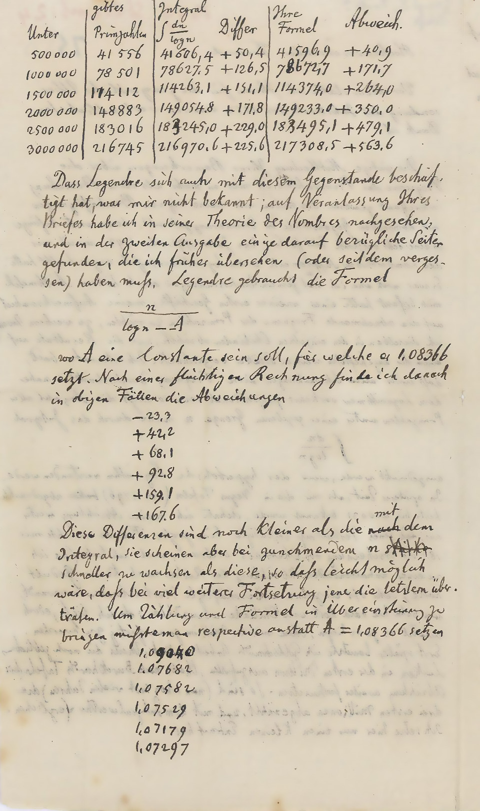
One of the brilliant aspects of the internet is how much easier it is to find source material of such things. Courtesy of the digitization center at the State and University Library of Göttingen (the university where Gauss worked), you can see a scan of the actual letter in question 4 .
In Figure 21.2.4, Gauss is comparing his calculations of the number of primes with his formula, as well as those of his correspondent and Legendre. Whether or not you can read Gauss' (quite legible) German, you can still note how in the last set of numbers he is essentially doing data science on Legendre's formula, with \(A\) as the modeling variable, using more and more detailed training sets!
Subsection 21.2.2 Exploring \(Li\)
Can we try for some more analysis? Since we saw that \(x/\log(x)\) didn't seem to be as good an approximation, we'll leave it out for now. This graphic show two representative 1000-wide stretches, and the following interact allows you to explore more of them.

Based on this evidence, it seems clear that \(Li(x)\text{,}\) even if it's a good approximation, should not ever be less than the actual count of primes. And yet, the English mathematician John Littlewood proved the following result.
Fact 21.2.6.
For any number \(x\text{,}\) there is an \(x'>x\) such that
Historical remark 21.2.7. Skewes' Number.
As remarkable as this seems, Littlewood's student Stanley Skewes proved the following even more amazing fact:
The first time this happens is no higher than
\begin{equation*} 10^{10^{10^{10^{1000}}}}\text{.} \end{equation*}
In Skewes' original paper, this bound had a \(34\) instead of \(1000\) in the last exponent 5 , but that result relied upon a special assumption (the so-called Riemann Hypothesis, see Chapter 25). Both of these bounds are known as Skewes' number.
We have known since the 1960's that there is an actual run of integers where \(Li\) is smaller starting near \(1.53\times 10^{1165}\text{.}\) Today we know that the first time this “switch” happens is no higher than \(1.4\times 10^{316}\) (see [E.7.23] and a follow-up from 2015 for the state of the art). Of course, we haven't even gotten remotely near those bounds with computers, although computation is necessary to help obtain these bounds.
This uncertainty sounds terrible, but actually is good news. After all, if \(\pi\) beats \(Li\) once in a while, then \(Li\) must be a great approximation indeed! So, just how great is it?